Seeing Probability
Bayes without the algebra
Give a room full of doctors this problem and most of them get it wrong, badly wrong, in a way that would frighten their patients. A disease affects 1 in 100 women. A test catches 90% of the women who have it, and raises a false alarm for 9% of the women who don’t. A patient tests positive. How likely is she to actually have the disease?
The common answer, from physicians, is around 90%. The real answer is about 9%. These are not careless people; they are experts, and the format of the question has beaten them.
Same problem, different clothes. Picture a thousand women. Ten of them have the disease, and nine of those ten test positive. Of the 990 who are healthy, about 89 test positive anyway. Lay the counts out in a grid:
| out of 1,000 women | test positive | test negative | total |
|---|---|---|---|
| has the disease | 9 | 1 | 10 |
| healthy | 89 | 901 | 990 |
| total | 98 | 902 | 1,000 |
Now the answer is just one number read against another. Of the 98 women who test positive, only nine are actually sick: nine out of ninety-eight, about one in ten. You did it in your head, and nothing changed but the format.
The problem is the format, not you
You are not bad at this. The percentages are.1 A figure like “90% sensitivity” or “9% false-positive rate” hides the one thing you need to see: how many actual people sit in each group. Your mind did not evolve doing percentages. It evolved counting things, and when you hand it counts instead of fractions, the answer falls out on its own.
That is the whole trick of seeing probability: stop computing and start counting. Replace the percentages with natural frequencies, real tallies of real cases, and a problem that defeats trained experts becomes something you can do at a stoplight.
Natural frequencies — counts of real cases (9 sick patients in 1,000; 80 good products among 260 yeses) instead of probabilities or percentages. The mind reasons far more reliably in counts than in fractions.
Build the tree
Put your own decision through it. Start with the population your product belongs to: the new products launched in a category like yours over a year, say a thousand IoT gadgets or a thousand new consumer apps. Most of them fail. Suppose that of every 1,000, only about 100 turn out to be genuinely wanted; the other 900 flop. That 100-in-1,000 is your base rate, the prior you carried in from the last chapters: one in ten. (The one-in-ten here is illustrative; the real figure varies by category and is notoriously slippery to pin down, so use the best number you can actually defend for yours.)
Base rate — how often something happens across a whole population, before you look at the one case in front of you. Here, 100 genuinely-wanted products in every 1,000: one in ten.
Now bring in the test. You’ve run a customer test on your product, and it’s a decent one: when a product is genuinely wanted, the test says “yes” 8 times in 10. But it isn’t perfect. When a product would actually flop, the test still says “yes” about 2 times in 10, because people are polite, or curious, or the test itself was leaky. Your product just got a “yes.” How likely is it to be one of the hundred that are genuinely wanted?
Don’t reach for a formula. Build a tree. Start with the thousand, split them by the base rate, split each branch by the test result, and count.
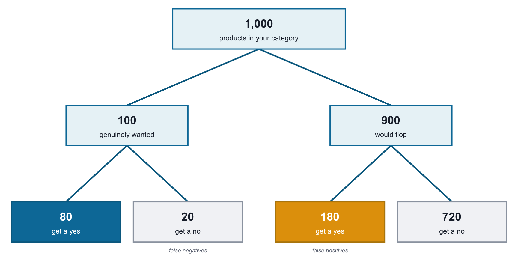
Now read it off the branches. A “yes” came back. How many products get a “yes” at all? Eighty of the genuinely-wanted ones, plus 180 of the flops: 260 in total. And of those 260, how many are actually any good? Just the 80. So a “yes” means good 80 times in 260 — about one in three.
Sit with that. A positive result on a test that catches 8 of every 10 good products still leaves you only about a third likely to have a good one. The “yes” was real evidence: it nearly tripled your odds, from 1 in 10 to roughly 1 in 3. That is genuine movement, not nothing. But a third is still a minority, and no single test hands a Bayesian certainty; it only makes you more or less sure. The reason you can see that at all is the base rate sitting in the tree, refusing to be forgotten.
The same thousand, made visible
If the tree shows the logic, a picture of the whole thousand shows the weight.

Each dot is one of the thousand products. The 260 that got a “yes” are the colored band across the top; everything grey got a “no.” Now look only at the color in that band. The blue, the genuinely good products the test correctly flagged, is a thin stripe. The gold, flops that got a “yes” anyway, is more than twice as thick. That gold is the base rate made visible: there are so many more flops to begin with that even a low false-alarm rate produces a flood of false yeses. Your one positive result is far more likely to be a drop in the gold than a drop in the blue.
This is the update
What you just did by counting is what a prior is for. The base rate, 1 in 10, was your prior. The “yes” was your evidence. The number you read off the tree, about 1 in 3, is your posterior: your belief after the evidence. You updated a prior into a posterior and never touched an equation.2
And notice what the picture would not let you do. It would not let you forget the base rate, because the base rate was the picture: the 100 against the 900, the blue against the gold. The doctors went wrong, and founders go wrong, in exactly the spot where the base rate drops out of view. Draw the tree and it cannot drop out, because you started by counting it.
One caution before you move on. A low posterior is not permission to ignore a result — a small chance of a catastrophe can still demand action, and what a belief is worth acting on depends on what is at stake. That coupling of odds with stakes is a later gate; here, the only task was to see the number clearly.
Worked example — Halo’s update, part by part
The same four pieces, on the venture we have been following. Halo’s question: will women switch from their phone to the ring?
- Prior — their honest starting belief before the interviews, built from two founders’ lived fear and the base rates of the space. Well-grounded on the problem (women feel unsafe), but only hopeful on the switch (that they would adopt a device).
- Evidence — a handful of interviews leaning their way.
- Likelihood — how much that evidence discriminates: whether a warm interview is likelier from a woman who would switch than from one who would not. Warm words come from both, so the interviews fit the two stories almost equally — a weak signal, like a test with a high false-yes rate.
- Posterior — the belief after the evidence: the prior nudged, not moved. A weak signal against a prior already carrying the weight leaves you close to where you started — enough to press on, not enough to build.
There is no new number here, because the decisive test is still ahead. But the shape is already clear: a soft likelihood and thin evidence leave the posterior sitting close to the prior. Which piece is which is the thing to hold onto — name them on your own decision and the arithmetic takes care of itself.
For the Curious — The formula you just avoided
There is an equation under all of this, and the counting you just did is that equation run on whole numbers instead of fractions. It is called Bayes’ theorem, and in words it says:
\[ \textsf{posterior} = \frac{\textsf{prior} \times \textsf{likelihood}}{\textsf{total probability of the evidence}} \]
Your prior is the base rate: how likely the product was to be good before the test, 1 in 10 (100 in 1000). The likelihood is how well a yes fits a genuinely good product, 8 in 10. The evidence in the denominator is every way a yes could arise: the good-and-yes cases plus the flop-and-yes cases. Drop your counts in and it is the arithmetic you already did: 80 / (80 + 180). The formula only says this — shift your belief in proportion to how well the evidence fits it, then rescale so the possibilities still add to one. Researchers teach it with counts not because the algebra is wrong but because almost no one reasons well in fractions.3 You never have to write the equation. But now you have seen it, and you can see it is only bookkeeping.
Learn From Your AI
I just learned to do Bayesian updating by counting cases out of 1,000. Now teach me Bayes’ theorem itself: what each part means and how my counting maps onto the formula. Start with one simple everyday example. Then, if I give you a base rate, a hit rate, and a false-positive rate, walk through my own numbers.
Trap to Avoid — The percentage that fools you
The test catches 80% of good products, so a “yes” means you’re 80% likely to be good — right? That is the mistake that beat the doctors. The 80% describes how the test treats good products; it is not the chance you’re good once you’ve gotten a yes. Those two numbers only match when the base rate is 50-50, which it almost never is. Whenever someone quotes you a single impressive percentage, ask the question the tree forces: out of how many, and against what base rate?
Working with your AI
Working with your AI — where you step in
Your AI will build this tree in seconds and do the counting flawlessly. Hand it the arithmetic. But the tree is only as honest as two numbers you have to supply, and the AI cannot find them for you.
- The base rate is yours. How often do products like yours actually succeed? That’s your prior from the last chapters, and a tree built on a flattering base rate lies cleanly and convincingly.
- The false-positive rate is yours too. Be honest about how often your test says “yes” to something that would flop. Optimists set it near zero; that’s how the amber disappears and the posterior lies.
- Read the posterior as movement, not verdict. The number tells you how far the evidence moved you, not whether you’ve arrived. Deciding whether it’s far enough is the next gate, not this one.
Ask Your AI
Build me a natural-frequency tree out of 1,000 for this decision: [state it]. My base rate is [X%], my test catches [Y%] of the true yeses, and it gives a false yes [Z%] of the time. Show me the four counts, tell me my posterior after a positive result, and flag which of my three numbers my answer is most sensitive to.
Putting It to Work
Try This — Draw your own thousand
Take a test you’re about to trust, and build the tree by hand.
- Start with 1,000 cases like yours.
- Split them by your base rate: how many of the thousand are the real thing?
- Split each group by the test: how many of the good ones pass, and how many of the rest pass anyway?
- Count the passes, and count how many of those passes are actually good. That ratio is your answer.
If the number startles you, the tree is working. It’s showing you the base rate your hopes had quietly deleted.
The move: When a result tempts you, don’t trust the percentage — draw the thousand. Split by the base rate, split by the test, and count the branch you care about. The posterior is a ratio you can see.
One thing in that tree should nag at you: a strong positive result still left you at only one in three, and the reason was the low base rate. When the base rate is low and the data is thin, the prior keeps its grip on the answer no matter how the evidence comes back. That is not a flaw in the method. It is the entrepreneur’s everyday condition, and it is where we turn next.
The idea that mathematical trouble is usually a failure of format rather than of the person, and that rigor can be made to feel like common sense extended, runs throughout Ellenberg (2014) — the animating spirit of this whole book.↩︎
For an accessible tour of how far this single move, updating a prior into a posterior, reaches across science and everyday life, see Chivers (2024).↩︎
The finding that natural-frequency formats make Bayesian reasoning intuitive, where percentages defeat even experts, is Gigerenzer and Hoffrage (1995); the general-audience case is Gigerenzer (2015).↩︎